Here are the steps to do this:
- Select the entire data set.
- Click the Home tab.
- In the Styles group, click on the ‘Conditional Formatting’ option.
- Hover the cursor on the Highlight Cell Rules option.
- Click on Duplicate Values.
- In the Duplicate Values dialog box, make sure ‘Duplicate’ is selected.
- Specify the formatting.
How do you reconcile data in Excel?
When it comes to reconciliation or matching the data VLOOKUP formula leads the table.
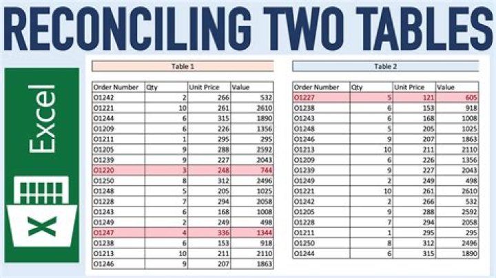
- For example, look at the below table.
- We have two data tables here, first one is Data 1 & the second one is Data 2.
- I have applied the SUM function for both the table’s Sale Amount column.
- Select the table array as Data 1 range.
How do you do intercompany reconciliation in Excel?
Powered by:
- Step 1: Create a data model: (No Worries, it’s already there for you)
- Step 2: Build a Hierarchy:
- Step 3: Paste your data into the Spreadsheet:
- Step 4: Reconcile your Intercompany Transactions:
- Step 5: Enjoy your Consolidated and Eliminated Reports.
How do I compare two sets of data in Excel?
To quickly highlight cells with different values in each individual row, you can use Excel’s Go To Special feature.
- Select the range of cells you want to compare.
- On the Home tab, go to Editing group, and click Find & Select > Go To Special… Then select Row differences and click the OK button.
How do you compare two data sets?
When you compare two or more data sets, focus on four features:
- Center. Graphically, the center of a distribution is the point where about half of the observations are on either side.
- Spread. The spread of a distribution refers to the variability of the data.
- Shape.
- Unusual features.
What are the steps of intercompany reconciliation?
For all three processes, you reconcile accounting documents in the following order:
- Data selection. You select documents across SAP systems and clients and transfer the data to the reconciliation database.
- Data assignment.
- Data reconciliation.
- Communication.
- Correction posting.
How do you compare two sets of data in a pivot table?
Excel: Use a Pivot Table to Compare Two Lists
- Add the heading Source in C1. Select C2:C21, type Forecast and press Ctrl+Enter to fill column C with the word Forecast.
- Change the heading in B1 to be Amount.
- Cut D2:E21 and paste just below the first list. Type Orders next to all of the List 2 records.
Are two sets of data statistically different?
No. A t-test tells you whether the difference between two sample means is “statistically significant” – not whether the two means are statistically different. A t-score with a p-value larger than 0.05 just states that the difference found is not “statistically significant”.
Can 2 pivot tables be linked?
Connect Another Pivot Table. If you create multiple pivot tables from the same pivot cache, you can connect them to the same slicers, and filter all the pivot tables at the same time. Select a cell in the second pivot table. On the Excel Ribbon’s Options tab, click Insert Slicer.
Can you do at test with 2 sets of data?
To perform a t-test your data needs to be continuous, have a normal distribution (or nearly normal) and the variance of the two sets of data needs to be the same (check out last week’s post to understand these terms better). You can use an unpaired t-test on paired data without a negative consequence.
How do I compare two Excel spreadsheets for missing data?
Compare 2 Excel workbooks
- Open the workbooks you want to compare.
- Go to the View tab, Window group, and click the View Side by Side button. That’s it!
What does it mean to say that figures should be reconciled?
Reconciliation is an accounting process that compares two sets of records to check that figures are correct and in agreement.
How do you compare two sets of data in Excel?
How to Complete an Excel ANOVA
- Recreate the columns using Excel.
- Go to Tools and select Data Analysis as shown.
- Click OK to the first choice, ANOVA: Single Factor.
- Click and drag your mouse from Pat’s name to the last score in Sheri’s column.
- Interpret the probability results by evaluating the F ratio.
What is the best way to compare two sets of data?
Common graphical displays (e.g., dotplots, boxplots, stemplots, bar charts) can be effective tools for comparing data from two or more data sets.
What is the formula of reconciliation?
A bank reconciliation can be thought of as a formula. The formula is (Cash account balance per your records) plus or minus (reconciling items) = (Bank statement balance). When you have this formula in balance, your bank reconciliation is complete. The difference between these two balances is due to reconciling items.
Can you compare two Excel files?
If you have two workbooks open in Excel that you want to compare, you can run Spreadsheet Compare by using the Compare Files command.
How do I find missing data in Excel using Vlookup?
Syntax of formula:
- VLOOKUP function looks up for the cell value in the 1st column of the table_array list.
- The ISNA function catches the #N/A error and returns TRUE if #N/A error exist or else returns FALSE.
- IF function returns “Is there” as Value if FALSE and “Missing” as value if TRUE.
How do you reconcile two lists in Excel?
Simply paste the summary data into the existing SummaryTable, the detail data into the DetailTable, and then right-click and Refresh the green results table. Excel instantly generates an updated reconciliation table, without any need to open the Query Editor!
How to prepare a reconciliation worksheet in Excel?
The basic steps to prepare the reconciliation worksheet are: 1 Create the summary query 2 Create the detail query 3 Create the reconciliation query
Is there a way to match two dates in Excel?
In Data 1, we have 12104 for the Date 04-Mar-2019, and in Data 2, we have 15104 for the same date, so there is a difference of 3000. Similarly, for the date 18-Mar-2019 in Data 1, we have 19351, and in Data 2, we have 10351, so the difference is 9000. For the same data, we can use the INDEX + MATCH function.
How to compare two lists or datasets in Excel?
Start by selecting the two columns of data. From the Home tab, select the Conditional Formatting drop down. Then select Highlight Cells Rules. Next select Duplicate values. A Duplicate Values settings box will open where you can define the formatting and select between Duplicate or Unique values.